Aperçu des variables
Les objets sf sont des data.frame.
Nous pouvons utiliser les fonctions head() ou summary().
#> Linking to GEOS 3.11.1, GDAL 3.6.2, PROJ 9.1.1; sf_use_s2() is TRUE
com <- st_read("data/lot.gpkg", layer = "communes", quiet = TRUE)
head(com, n = 3)
#> Simple feature collection with 3 features and 12 fields
#> Geometry type: MULTIPOLYGON
#> Dimension:     XY
#> Bounding box:  xmin: 557759.2 ymin: 6371852 xmax: 607179 ymax: 6418606
#> Projected CRS: RGF93 v1 / Lambert-93
#>   INSEE_COM  NOM_COM         STATUT POPULATION     AGR_H    AGR_F     IND_H
#> 1     46001    Albas Commune simple        522  4.978581 0.000000  4.936153
#> 2     46002   Albiac Commune simple         67  0.000000 9.589041  0.000000
#> 3     46003 Alvignac Commune simple        706 10.419682 0.000000 10.419682
#>      IND_F     BTP_H BTP_F     TER_H     TER_F                           geom
#> 1 0.000000  9.957527     0 44.917145 34.681799 MULTIPOLYGON (((559262 6371...
#> 2 0.000000  4.794521     0  4.794521  9.589041 MULTIPOLYGON (((605540.7 64...
#> 3 5.209841 10.419682     0 57.308249 78.147612 MULTIPOLYGON (((593707.7 64...
#>   INSEE_COM           NOM_COM             STATUT            POPULATION
#>  Length:313         Length:313         Length:313         Min.   :   49.0
#>  Class :character   Class :character   Class :character   1st Qu.:  172.0
#>  Mode  :character   Mode  :character   Mode  :character   Median :  300.0
#>                                                           Mean   :  555.7
#>                                                           3rd Qu.:  529.0
#>                                                           Max.   :19907.0
#>      AGR_H            AGR_F            IND_H             IND_F
#>  Min.   : 0.000   Min.   : 0.000   Min.   :  0.000   Min.   :  0.000
#>  1st Qu.: 0.000   1st Qu.: 0.000   1st Qu.:  4.843   1st Qu.:  0.000
#>  Median : 5.000   Median : 0.000   Median :  5.516   Median :  4.943
#>  Mean   : 6.935   Mean   : 2.594   Mean   : 16.395   Mean   :  7.635
#>  3rd Qu.:10.013   3rd Qu.: 5.000   3rd Qu.: 19.715   3rd Qu.:  9.905
#>  Max.   :56.179   Max.   :24.641   Max.   :602.867   Max.   :184.016
#>      BTP_H             BTP_F             TER_H             TER_F
#>  Min.   :  0.000   Min.   : 0.0000   Min.   :   0.00   Min.   :   0.00
#>  1st Qu.:  0.000   1st Qu.: 0.0000   1st Qu.:  10.00   1st Qu.:  15.15
#>  Median :  5.000   Median : 0.0000   Median :  20.00   Median :  30.26
#>  Mean   :  9.572   Mean   : 0.9723   Mean   :  42.17   Mean   :  60.77
#>  3rd Qu.: 10.329   3rd Qu.: 0.0000   3rd Qu.:  44.69   3rd Qu.:  63.95
#>  Max.   :203.122   Max.   :16.9238   Max.   :1778.87   Max.   :2397.18
#>             geom
#>  MULTIPOLYGON :313
#>  epsg:2154    :  0
#>  +proj=lcc ...:  0
#>
#>
#>
Pour transformer un objet sf en simple data.frame (sans géométries), nous pouvons utiliser les fonctions st_set_geometry() ou st_drop_geometry().
com_df1 <- st_set_geometry(com, NULL)
com_df2 <- st_drop_geometry(com)
identical(com_df1, com_df2)
#>   INSEE_COM  NOM_COM         STATUT POPULATION     AGR_H    AGR_F     IND_H
#> 1     46001    Albas Commune simple        522  4.978581 0.000000  4.936153
#> 2     46002   Albiac Commune simple         67  0.000000 9.589041  0.000000
#> 3     46003 Alvignac Commune simple        706 10.419682 0.000000 10.419682
#>      IND_F     BTP_H BTP_F     TER_H     TER_F
#> 1 0.000000  9.957527     0 44.917145 34.681799
#> 2 0.000000  4.794521     0  4.794521  9.589041
#> 3 5.209841 10.419682     0 57.308249 78.147612
Affichage
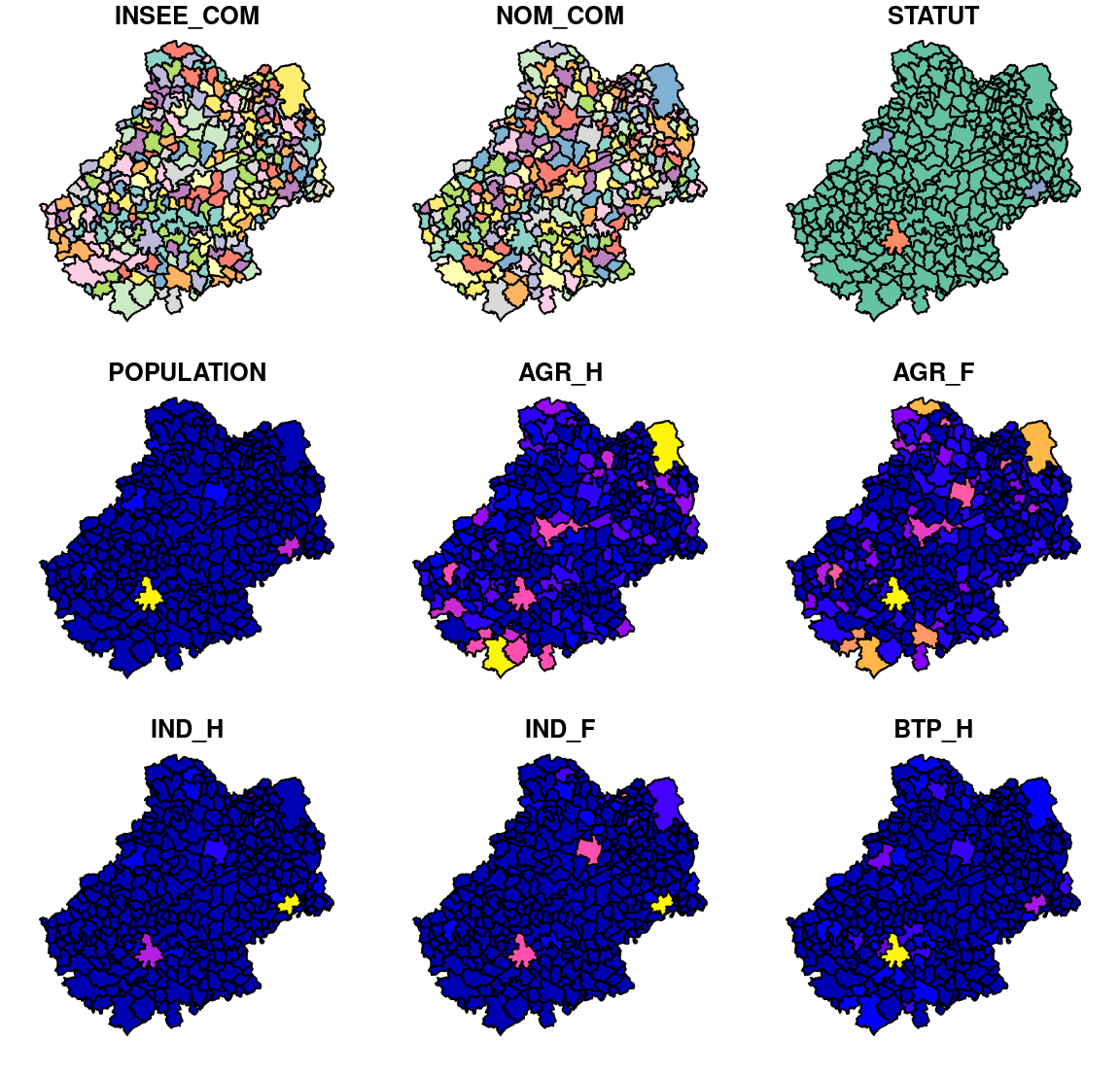
Aperçu des variables avec plot() :
#> Warning: plotting the first 9 out of 12 attributes; use max.plot = 12 to plot
#> all
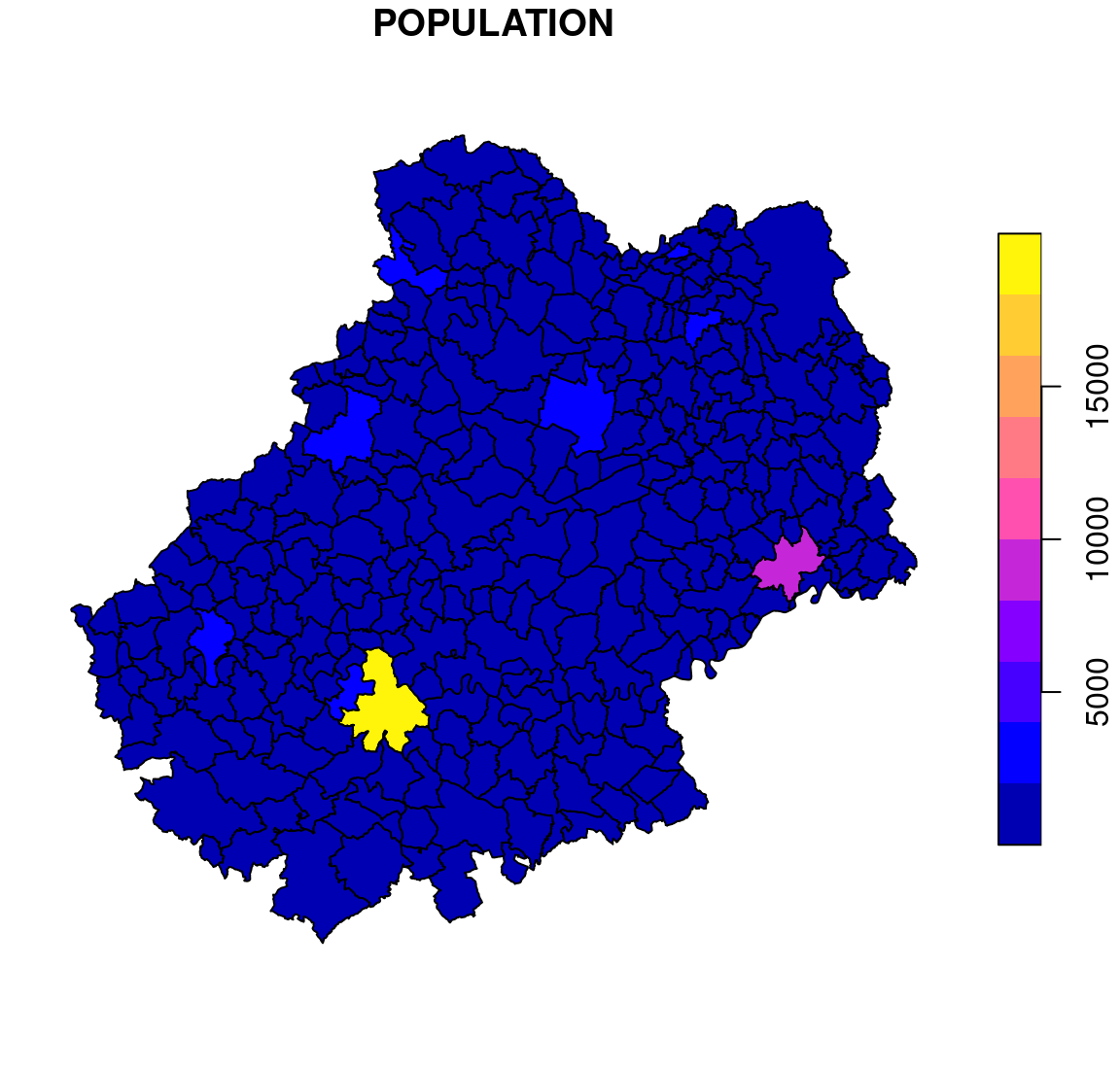
Affichage d’une seule variable :
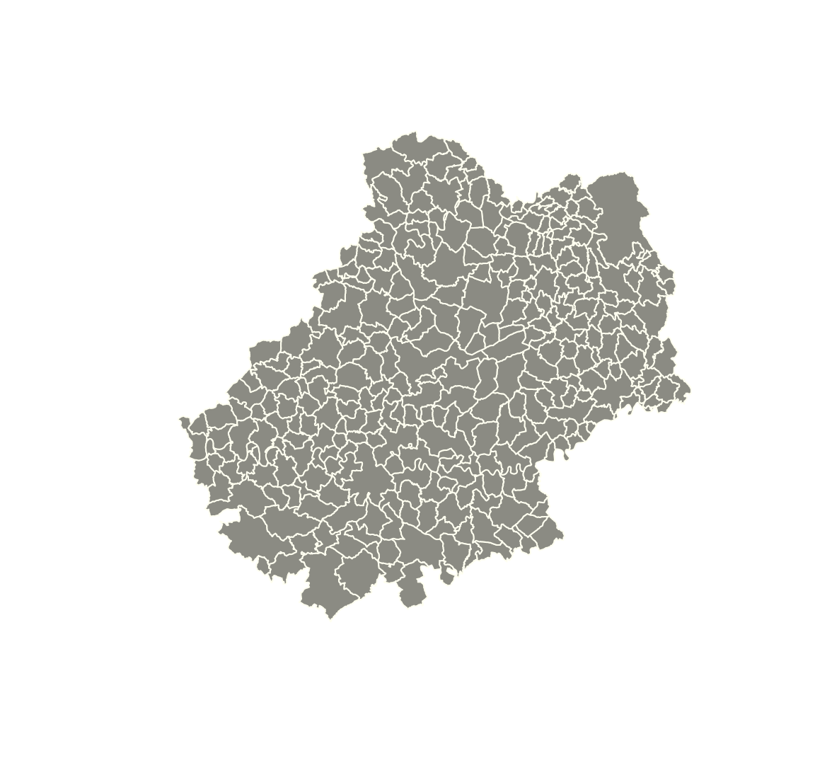
Affichage de la géométrie seule :
plot(st_geometry(com), col = "ivory4", border = "ivory")
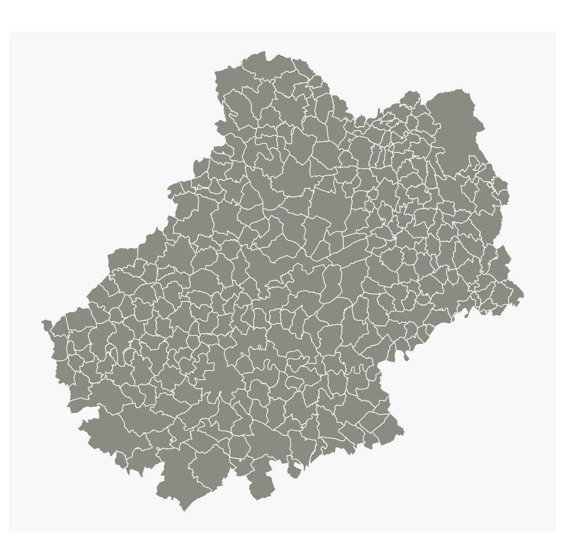
Il est aussi possible d’utiliser le package mapsf (Giraud, 2023) pour afficher les objets sf.
library(mapsf)
mf_map(com, col = "ivory4", border = "ivory")