In this chapter, we will briefly describe a few geometric operations made available by the sf package, on vector data.
3.1 Spatial selection and join
3.1.1 Spatial selection
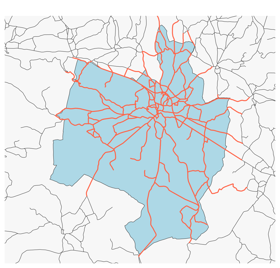
st_filter() is used to perform spatial selections. The .predicate argument lets you pick the selection criterion by using one of the “geometric predicate” functions (e.g. st_intersects(), st_within(), st_crosses()…).
Here, we select the roads that intersect the municipality of Gramat. We do not modify their geometry.
Import the layers of municipalities and restaurants.
Perform a spatial join to find the name and identifier of the municipality where each restaurant is located.
3.2 Geometrical operations
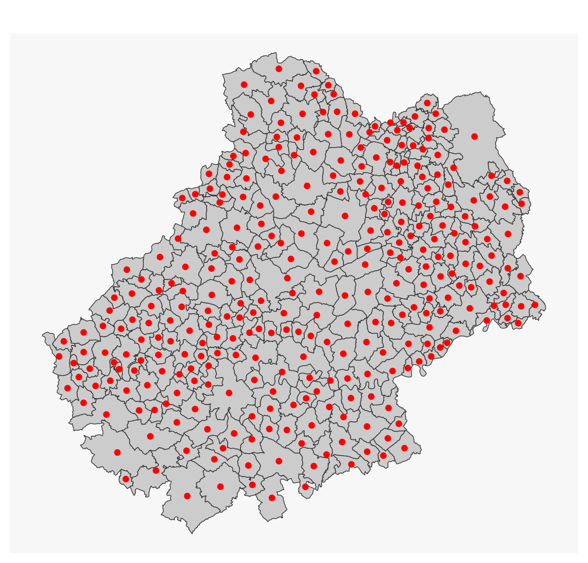
3.2.1 Centroids
mun_c <-st_centroid(mun)
#> Warning: st_centroid assumes attributes are constant over geometries
mf_map(mun)mf_map(mun_c, add =TRUE, cex =1.2, col ="red", pch =20)
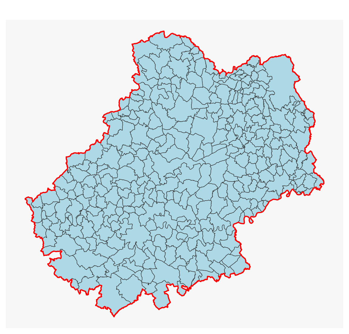
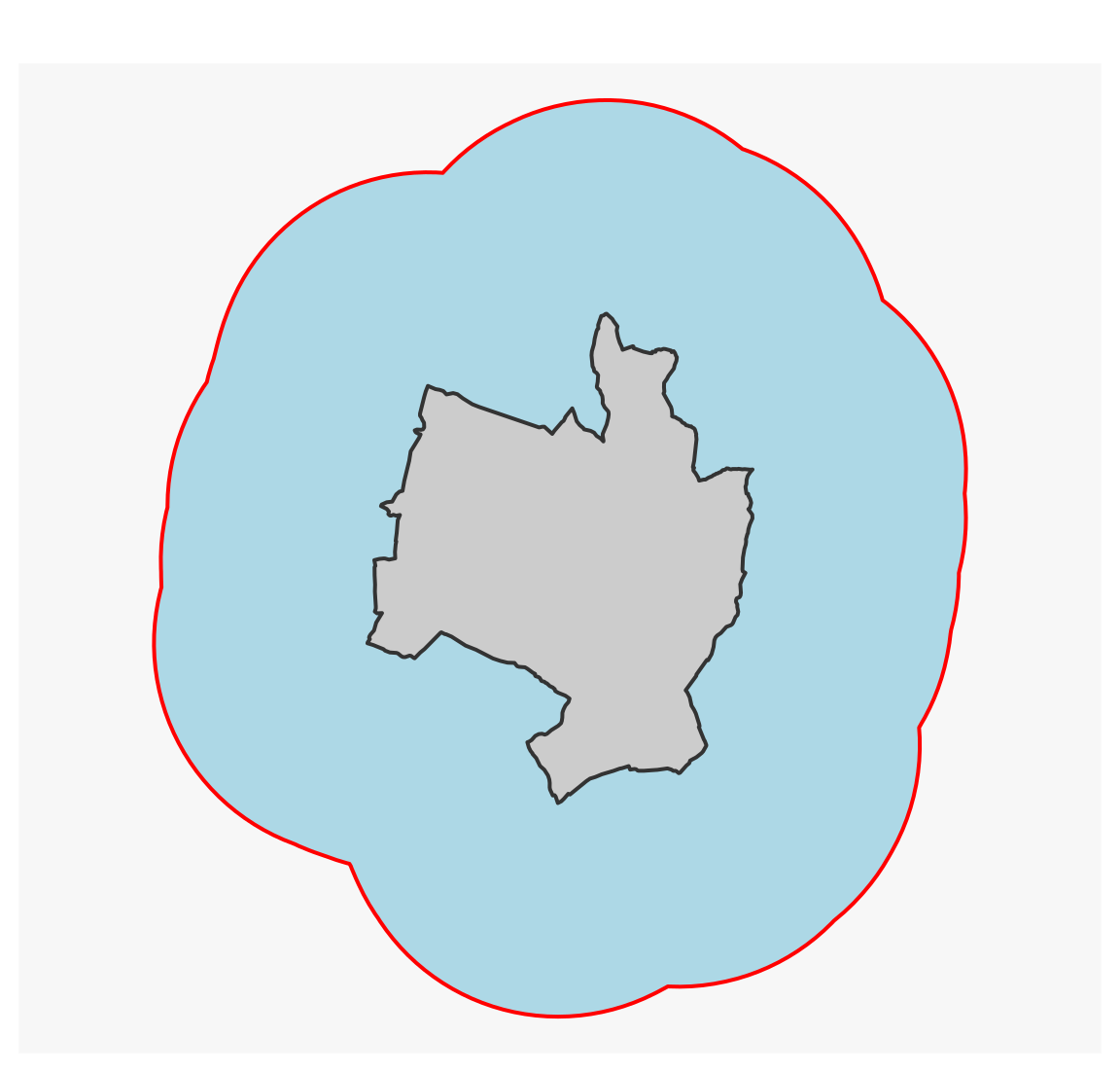
3.2.2 Aggregate polygons
dep_46 <-st_union(mun)mf_map(mun, col ="lightblue")mf_map(dep_46, col =NA, border ="red", lwd =2, add =TRUE)
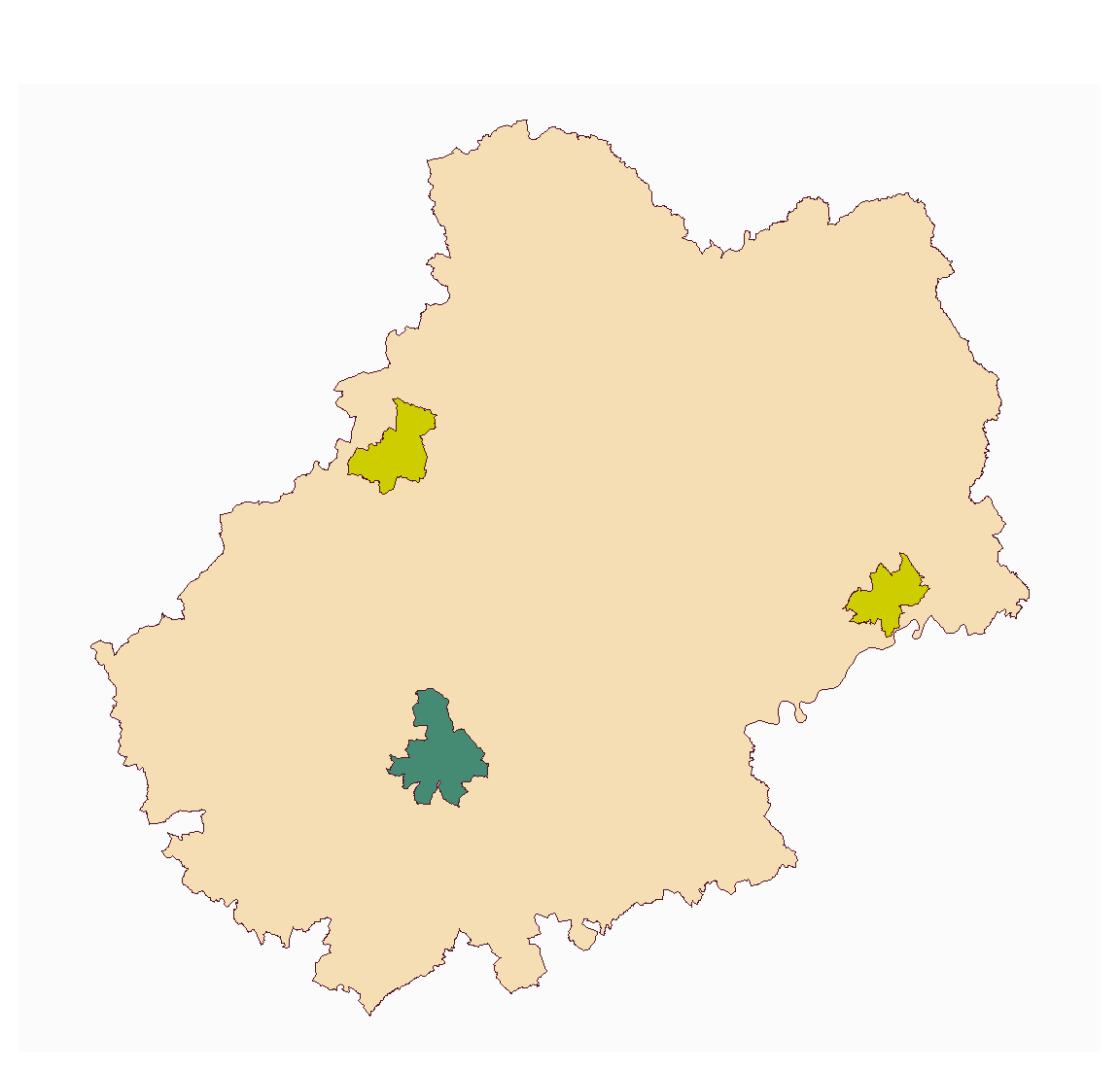
3.2.3 Aggregate polygons using a grouping variable
In this example, we aggregate polygons according to their hierarchical status (simple municipality, subprefecture, prefecture). We can aggregate the geometries (union) as well as their attributes (sum of population).
# Grouping variablei <- mun$STATUT mun_u <-st_sf(STATUT =tapply(X = mun$STATUT , INDEX = i, FUN = head, 1),POPULATION =tapply(X = mun$POPULATION , INDEX = i, FUN = sum), geometry =tapply(X = mun , INDEX = i, FUN = st_union), crs =st_crs(mun)) mun_u
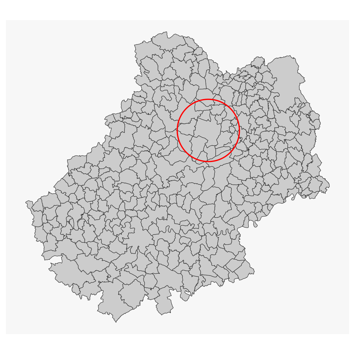
Using st_intersection(), we can cut one layer by another. Here, geometries are modified.
# create a buffer zone around the centroid of Gramatzone <-st_geometry(gramat) |>st_centroid() |>st_buffer(10000)mf_map(mun)mf_map(zone, border ="red", col =NA, lwd =2, add =TRUE)
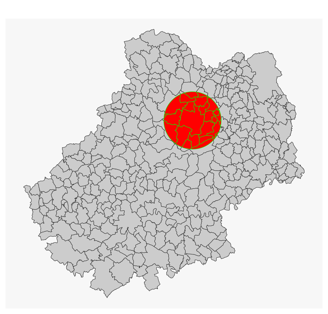
mun_z <-st_intersection(x = mun, y = zone)
#> Warning: attribute variables are assumed to be spatially constant throughout
#> all geometries
mf_map(mun)mf_map(mun_z, col ="red", border ="green", add =TRUE)
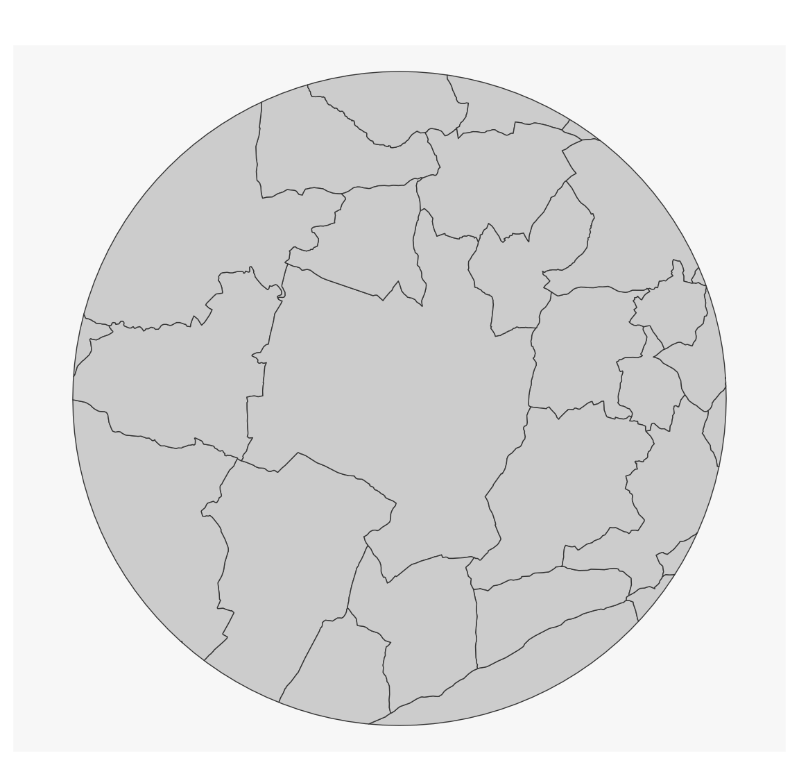
mf_map(mun_z)
In this example, we’ve used pipes (|>). Pipes are used to concatenate a sequence of instructions.
3.2.6 Regular grid
st_make_grid() is used to create a regular grid. It produces an sfc object, and then you need to use st_sf() to transform this sfc object into an sf object. We also add a column of unique identifiers.
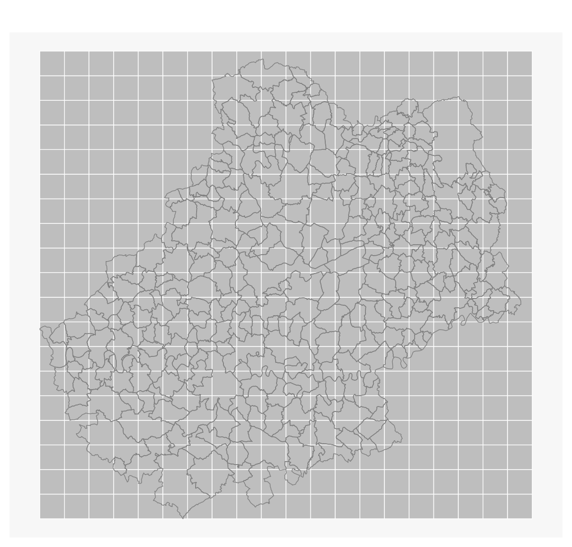
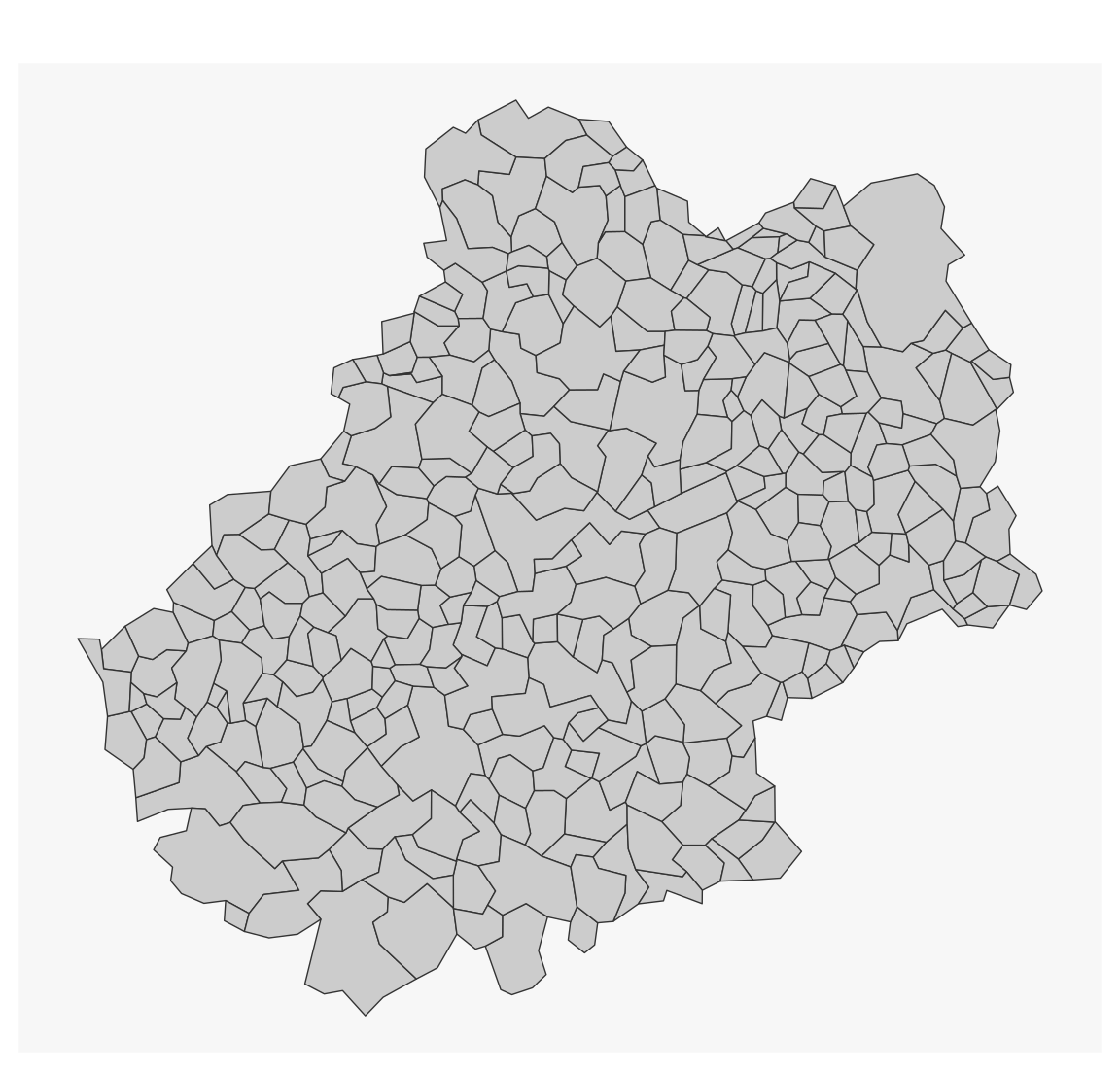
# create a gridgrid <-st_make_grid(x = mun, cellsize =5000)# transform to sf, add identifiergrid <-st_sf(ID =1:length(grid), geom = grid)mf_map(grid, col ="grey", border ="white")mf_map(mun, col =NA, border ="grey50", add =TRUE)
When working with European data or at EU scale, check the gridmaker package (Kotov 2025) in order to create GISCO compatible and INSPIRE-compliant grids.
3.2.7 Counting points in polygons
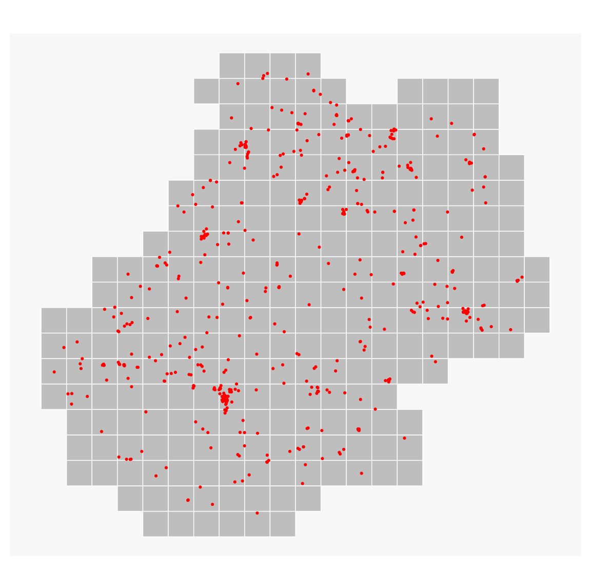
Select the grid tiles which intersect the department with st_filter().
We then use st_intersects(..., sparse = TRUE), which will produce a list of the elements of the restaurant object inside each element of the grid object (via their indexes).
inter <-st_intersects(grid, restaurant, sparse =TRUE)length(inter) ==nrow(grid)
#> [1] TRUE
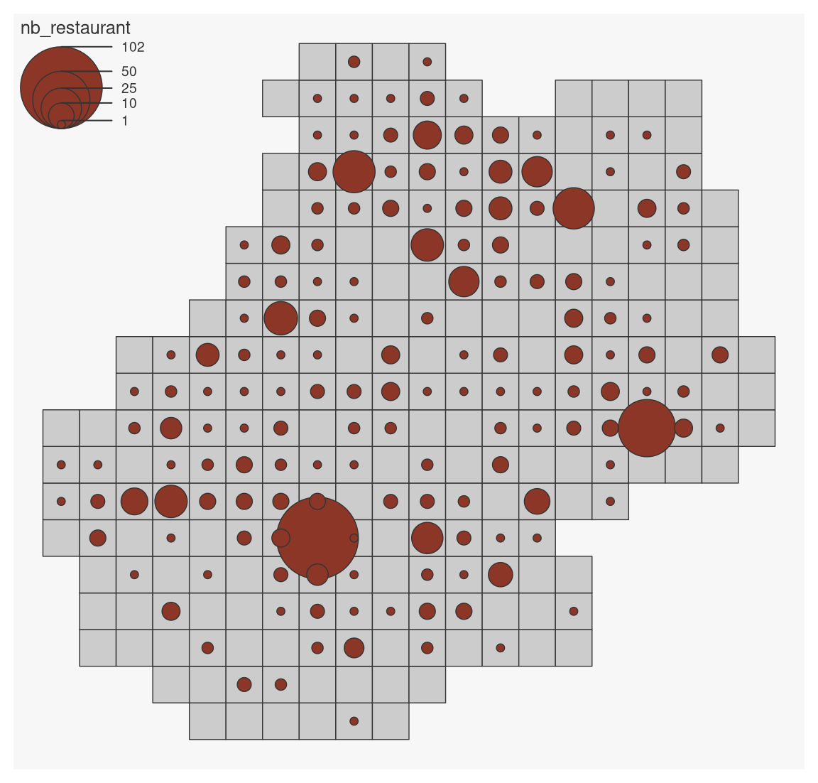
To count the number of restaurants, all we need to do is report the length of each of the elements in this list.
grid$nb_restaurant <-lengths(inter)mf_map(grid)mf_map(grid, var ="nb_restaurant", type ="prop")
#> 94 '0' values are not plotted on the map.
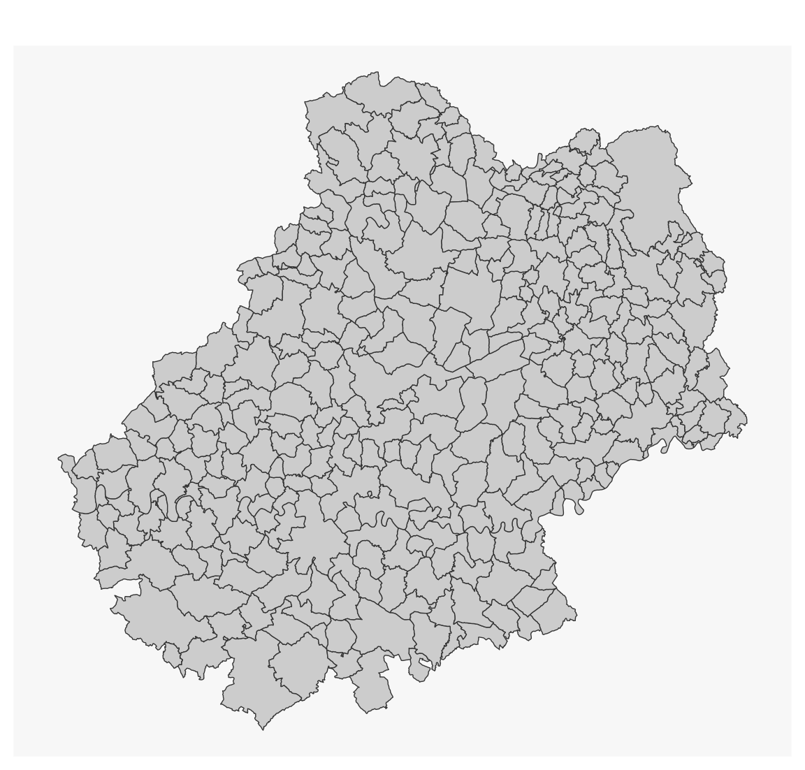
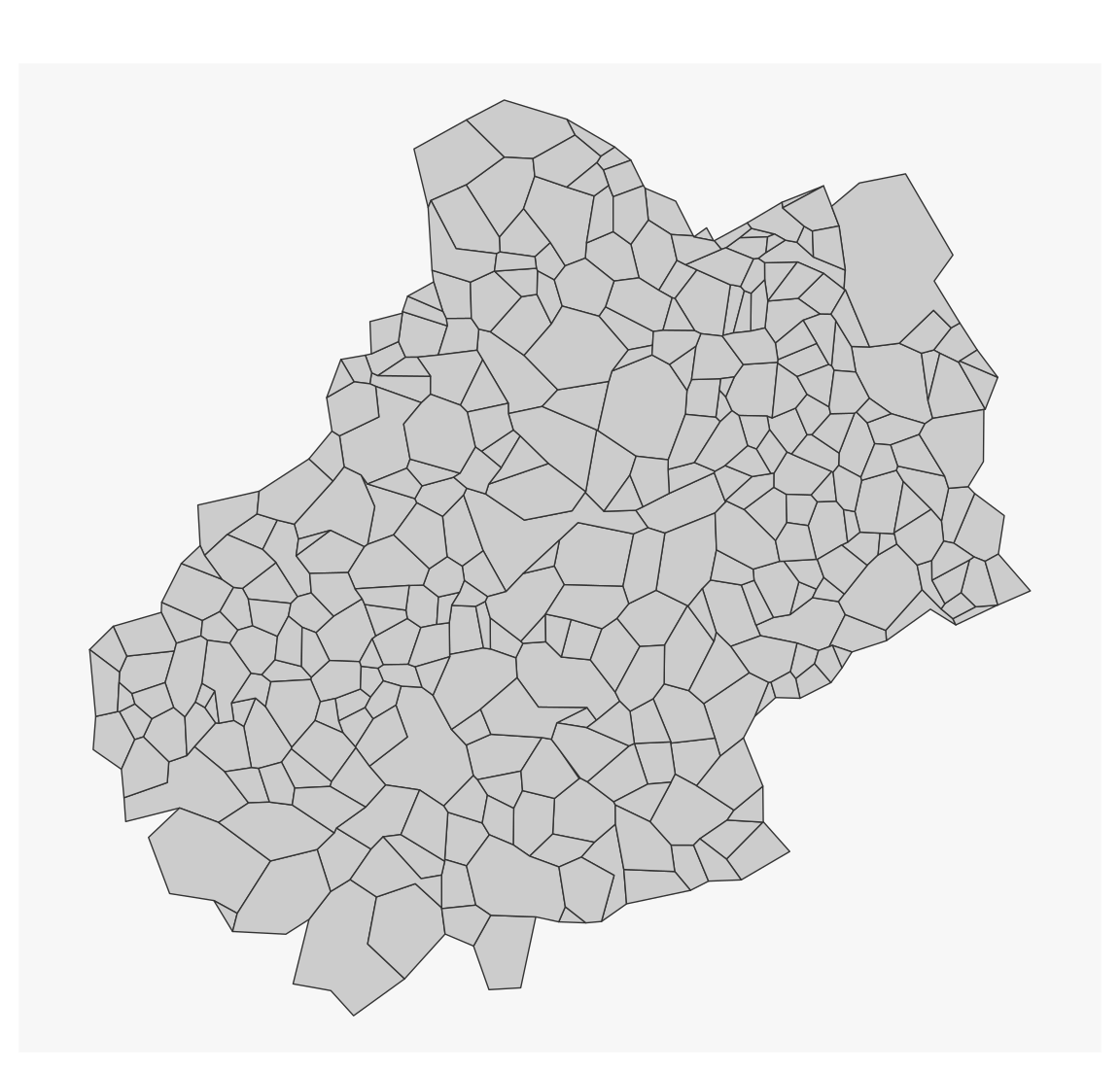
3.2.8 Geometries simplification
The rmapshaper package (Teucher and Russell 2025) builds on the Mapshaper JavaScript library (Bloch 2013) to offer several topology-friendly methods for simplifying geometries.
The keep argument is used to indicate the level of simplification. The keep_shapes argument is used to keep all polygons when the simplification level is high.