3 Manipuler les données vectorielles

3.1 Format des objets spatiaux `sf`

Les objets sf sont des data.frame dont l’une des colonnes contient des géométries. Cette colonne est de la classe sfc (simple feature column) et chaque individu de la colonne est un sfg (simple feature geometry).
Ce format est très pratique dans la mesure ou les données et les géométries sont intrinsèquement liées dans un même objet.

Vignette décrivant le format simple feature

Simple Features for R

3.2 Import et export de données

Les fonctions st_read() et st_write() permettent d’importer et d’exporter de nombreux types de fichiers.
Les lignes suivantes importent la couche des communes du département du Lot situé dans le fichier geopackage lot46.gpkg.

library(sf)

#> Linking to GEOS 3.9.0, GDAL 3.2.2, PROJ 7.2.1; sf_use_s2() is TRUE

com <- st_read("data/lot46.gpkg", layer = "commune")

#> Reading layer `commune' from data source 
#>   `/home/tim/Documents/prz/ined2022/data/lot46.gpkg' using driver `GPKG'
#> Simple feature collection with 313 features and 12 fields
#> Geometry type: MULTIPOLYGON
#> Dimension:     XY
#> Bounding box:  xmin: 539668.5 ymin: 6346290 xmax: 637380.9 ymax: 6439668
#> Projected CRS: RGF93 / Lambert-93

Les lignes suivantes exportent l’objet com dans un dossier data aux formats geopackage et shapefile.

st_write(obj = com, dsn = "data/com.gpkg", layer = "commune", delete_layer = TRUE)

#> Deleting layer `commune' using driver `GPKG'
#> Writing layer `commune' to data source `data/com.gpkg' using driver `GPKG'
#> Writing 313 features with 12 fields and geometry type Multi Polygon.

st_write(obj = com, "data/com.shp", layer_options = "ENCODING=UTF-8", delete_layer = TRUE)

#> Deleting layer `com' using driver `ESRI Shapefile'
#> Writing layer `com' to data source `data/com.shp' using driver `ESRI Shapefile'
#> options:        ENCODING=UTF-8 
#> Writing 313 features with 12 fields and geometry type Multi Polygon.

3.3 Affichage

Aperçu des variables via les fonctions head() et plot().

head(com)

#> Simple feature collection with 6 features and 12 fields
#> Geometry type: MULTIPOLYGON
#> Dimension:     XY
#> Bounding box:  xmin: 556391.9 ymin: 6371852 xmax: 614866.5 ymax: 6418606
#> Projected CRS: RGF93 / Lambert-93
#>   INSEE_COM         NOM_COM         STATUT POPULATION     AGR_H    AGR_F
#> 1     46001           Albas Commune simple        522  4.978581 0.000000
#> 2     46002          Albiac Commune simple         67  0.000000 9.589041
#> 3     46003        Alvignac Commune simple        706 10.419682 0.000000
#> 4     46004         Anglars Commune simple        219  0.000000 0.000000
#> 5     46005 Anglars-Juillac Commune simple        329  4.894895 4.894895
#> 6     46006   Anglars-Nozac Commune simple        377  4.840849 0.000000
#>       IND_H     IND_F     BTP_H    BTP_F     TER_H     TER_F
#> 1  4.936153  0.000000  9.957527 0.000000 44.917145 34.681799
#> 2  0.000000  0.000000  4.794521 0.000000  4.794521  9.589041
#> 3 10.419682  5.209841 10.419682 0.000000 57.308249 78.147612
#> 4 20.000000 15.000000 10.000000 0.000000 20.000000 20.000000
#> 5  4.894895  0.000000  0.000000 0.000000 29.369369 29.369369
#> 6  0.000000  0.000000  9.681698 4.840849 43.567639 38.726790
#>                             geom
#> 1 MULTIPOLYGON (((559262 6371...
#> 2 MULTIPOLYGON (((605540.7 64...
#> 3 MULTIPOLYGON (((593707.7 64...
#> 4 MULTIPOLYGON (((613211.3 64...
#> 5 MULTIPOLYGON (((556744.9 63...
#> 6 MULTIPOLYGON (((576667.2 64...

plot(com)

#> Warning: plotting the first 9 out of 12 attributes; use max.plot = 12 to plot
#> all

Affichage de la géométrie uniquement.

plot(st_geometry(com))

3.4 Les systèmes de coordonnées

3.4.1 Consulter le système de coordonnées d’un objet

La fonction st_crs() permet de consulter le système de coordonnées utilisé par un objet sf.

st_crs(com)

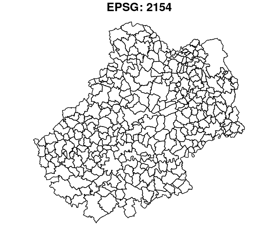
#> Coordinate Reference System:
#>   User input: RGF93 / Lambert-93 
#>   wkt:
#> PROJCRS["RGF93 / Lambert-93",
#>     BASEGEOGCRS["RGF93",
#>         DATUM["Reseau Geodesique Francais 1993",
#>             ELLIPSOID["GRS 1980",6378137,298.257222101,
#>                 LENGTHUNIT["metre",1]]],
#>         PRIMEM["Greenwich",0,
#>             ANGLEUNIT["degree",0.0174532925199433]],
#>         ID["EPSG",4171]],
#>     CONVERSION["Lambert-93",
#>         METHOD["Lambert Conic Conformal (2SP)",
#>             ID["EPSG",9802]],
#>         PARAMETER["Latitude of false origin",46.5,
#>             ANGLEUNIT["degree",0.0174532925199433],
#>             ID["EPSG",8821]],
#>         PARAMETER["Longitude of false origin",3,
#>             ANGLEUNIT["degree",0.0174532925199433],
#>             ID["EPSG",8822]],
#>         PARAMETER["Latitude of 1st standard parallel",49,
#>             ANGLEUNIT["degree",0.0174532925199433],
#>             ID["EPSG",8823]],
#>         PARAMETER["Latitude of 2nd standard parallel",44,
#>             ANGLEUNIT["degree",0.0174532925199433],
#>             ID["EPSG",8824]],
#>         PARAMETER["Easting at false origin",700000,
#>             LENGTHUNIT["metre",1],
#>             ID["EPSG",8826]],
#>         PARAMETER["Northing at false origin",6600000,
#>             LENGTHUNIT["metre",1],
#>             ID["EPSG",8827]]],
#>     CS[Cartesian,2],
#>         AXIS["easting (X)",east,
#>             ORDER[1],
#>             LENGTHUNIT["metre",1]],
#>         AXIS["northing (Y)",north,
#>             ORDER[2],
#>             LENGTHUNIT["metre",1]],
#>     USAGE[
#>         SCOPE["Engineering survey, topographic mapping."],
#>         AREA["France - onshore and offshore, mainland and Corsica."],
#>         BBOX[41.15,-9.86,51.56,10.38]],
#>     ID["EPSG",2154]]

3.4.2 Modifier le système de coordonnées d’un objet

La fonction st_transform() permet de change le système de coordonnées d’un objet sf, de le reprojeter.

plot(st_geometry(com))
title("EPSG: 2154")

com_reproj <- st_transform(com, "epsg:3035")
plot(st_geometry(com_reproj))
title("EPSG: 3035")

Le site Spatial Reference met à disposition les références de très nombreux systèmes de coordonnées.

3.5 Sélection par attributs

Les objets sf sont des data.frame, on peut donc sélectionner leur lignes et leur colonnes de la même manière que les data.frame.

# selection de ligne
com[1:2, ]

#> Simple feature collection with 2 features and 12 fields
#> Geometry type: MULTIPOLYGON
#> Dimension:     XY
#> Bounding box:  xmin: 557759.2 ymin: 6371852 xmax: 607179 ymax: 6410204
#> Projected CRS: RGF93 / Lambert-93
#>   INSEE_COM NOM_COM         STATUT POPULATION    AGR_H    AGR_F    IND_H IND_F
#> 1     46001   Albas Commune simple        522 4.978581 0.000000 4.936153     0
#> 2     46002  Albiac Commune simple         67 0.000000 9.589041 0.000000     0
#>      BTP_H BTP_F     TER_H     TER_F                           geom
#> 1 9.957527     0 44.917145 34.681799 MULTIPOLYGON (((559262 6371...
#> 2 4.794521     0  4.794521  9.589041 MULTIPOLYGON (((605540.7 64...

com[com$NOM_COM == "Gramat", ]

#> Simple feature collection with 1 feature and 12 fields
#> Geometry type: MULTIPOLYGON
#> Dimension:     XY
#> Bounding box:  xmin: 593605.6 ymin: 6402330 xmax: 602624.6 ymax: 6413784
#> Projected CRS: RGF93 / Lambert-93
#>     INSEE_COM NOM_COM         STATUT POPULATION    AGR_H    AGR_F    IND_H
#> 119     46128  Gramat Commune simple       3468 10.19868 15.29802 122.3842
#>        IND_F    BTP_H BTP_F    TER_H    TER_F                           geom
#> 119 107.0862 56.09275     0 260.0664 304.1941 MULTIPOLYGON (((594713.1 64...

# selection de colonnes
com[com$NOM_COM == "Gramat", 1:4]

#> Simple feature collection with 1 feature and 4 fields
#> Geometry type: MULTIPOLYGON
#> Dimension:     XY
#> Bounding box:  xmin: 593605.6 ymin: 6402330 xmax: 602624.6 ymax: 6413784
#> Projected CRS: RGF93 / Lambert-93
#>     INSEE_COM NOM_COM         STATUT POPULATION                           geom
#> 119     46128  Gramat Commune simple       3468 MULTIPOLYGON (((594713.1 64...

3.6 Sélection spatiale

3.6.1 Intersections

Sélection des routes intesectant la commune de Gramat.

route <- st_read("data/lot46.gpkg", layer = "route", quiet = TRUE)
gramat <-  com[com$NOM_COM == "Gramat", ]
inter <- st_intersects(x = route, y = gramat, sparse = FALSE)
head(inter)

#>       [,1]
#> [1,] FALSE
#> [2,] FALSE
#> [3,] FALSE
#> [4,] FALSE
#> [5,] FALSE
#> [6,] FALSE

dim(inter)

#> [1] 16096     1

L’objet inter est une matrice qui indique pour chacun des éléments de l’objet route (16096 éléments) si il intersecte chacun des élément de l’objet gramat (1 élément). La dimension de la matrice est donc bien 16096 lignes * 1 colonne.
Notez l’utilisation du paramètre sparse = FALSE ici. Il est ensuite possible de créer une colonne à partir de cet objet :

route$intersect_gramat <- inter
plot(st_geometry(gramat), col = "lightblue")
plot(st_geometry(route), add = TRUE)
plot(st_geometry(route[route$intersect_gramat, ]), 
     col = "tomato", lwd = 2, add = TRUE)

3.6.2 Contains / Within

Sélection des routes contenues dans la commune de Gramat. La fonctin st_within() fonctionne comme la fonction st_intersects()

route$within_gramat <- st_within(route, gramat, sparse = FALSE)
plot(st_geometry(gramat), col = "lightblue")
plot(st_geometry(route), add = TRUE)
plot(st_geometry(route[route$within_gramat, ]), col = "tomato", 
     lwd = 2, add = TRUE)

3.7 Opérations sur les géométries

3.7.1 Extraire des centroides

com_c <- st_centroid(com)

#> Warning in st_centroid.sf(com): st_centroid assumes attributes are constant over
#> geometries of x

plot(st_geometry(com))
plot(st_geometry(com_c), add = TRUE, col = "red", cex = .5, pch = 20)

3.7.2 Agréger des polygones

dep_46 <- st_union(com)
plot(st_geometry(com), col = "lightblue")
plot(st_geometry(dep_46), add = TRUE, lwd = 1.2, border = "red")

3.7.3 Agréger des polygones en fonction d’une variable

com_u <- aggregate(x = com[,c("POPULATION")],
                   by = list(STATUT = com$STATUT),
                   FUN = "sum")
plot(com_u)

3.7.4 Construire une zone tampon

gramat_b <- st_buffer(x = gramat, dist = 5000)
plot(st_geometry(gramat_b), col = "lightblue", lwd=2, border = "red")
plot(st_geometry(gramat), add = TRUE, lwd = 2)

3.7.5 Réaliser une intersection

En utilisant la fonction st_intersection() on va découper une couche par une autre.

# création d'une zone tampon autour du centroid de la commune de Gramat
# en utilisant le pipe
zone <- st_geometry(gramat) |>
  st_centroid() |>
  st_buffer(10000)
plot(st_geometry(com))
plot(zone, border = "red", lwd = 2, add = TRUE)

com_z <- st_intersection(x = com, y = zone)

#> Warning: attribute variables are assumed to be spatially constant throughout all
#> geometries

plot(st_geometry(com))
plot(st_geometry(com_z), col="red", border="green", add=T)

plot(st_geometry(com_z))

3.8 Mesures

3.8.1 Créer une matrice de distances

Si le système de projection du jeu de données est renseigné les distances sont exprimées dans l’unité de mesure de la projection (en mètres le plus souvent).

mat <- st_distance(x = com_c, y = com_c)
mat[1:5,1:5]

#> Units: [m]
#>           [,1]     [,2]     [,3]     [,4]      [,5]
#> [1,]     0.000 56784.77 54353.94 61166.42  3790.688
#> [2,] 56784.770     0.00 12454.29  7146.11 57288.103
#> [3,] 54353.942 12454.29     0.00 19388.52 54030.811
#> [4,] 61166.418  7146.11 19388.52     0.00 62016.141
#> [5,]  3790.688 57288.10 54030.81 62016.14     0.000

3.9 Exercice

Importer la couche des communes du département du Lot et la couche des restaurants à partir du fichier geopackage lot46.gpkg.

La fonction st_layers() permet de connaître les couches présentes dans un geopackage.

library(sf)
st_layers('data/lot46.gpkg')

#> Driver: GPKG 
#> Available layers:
#>    layer_name geometry_type features fields           crs_name
#> 1 departement Multi Polygon       96      5 RGF93 / Lambert-93
#> 2     commune Multi Polygon      313     12 RGF93 / Lambert-93
#> 3       route   Line String    16096     17 RGF93 / Lambert-93
#> 4  restaurant         Point     4734     12 RGF93 / Lambert-93

com <- st_read("data/lot46.gpkg", layer = 'commune', quiet = TRUE)
resto <- st_read("data/lot46.gpkg", layer = 'restaurant', quiet = TRUE)

Afficher la couche des communes (fond gris, bordures en blanc) et la couche des restaurants (petits cercles, fond rouge, contours en blanc) sur une même carte.

Rappel : La fonction st_geometry() permet d’accéder à la géométrie d’un objet sf.

plot(st_geometry(com), col = "grey", border = "white")
plot(st_geometry(resto), pch = 21, cex = .5, bg = "red", 
     col = "white", add = TRUE)

Sélectionner la commune de Cahors et assigner le résultat dans un objet cahors.

cahors <- com[com$NOM_COM == "Cahors", ]

Combien de restaurants se trouvent à Cahors ou à moins de 10 km de Cahors?

sum(st_distance(x = resto, y = cahors) <= units::as_units(10, 'km'))

#> [1] 162

nrow(resto[st_buffer(cahors, 10000), ])

#> [1] 162

nrow(st_intersection(resto, st_buffer(cahors, 10000)))

#> Warning: attribute variables are assumed to be spatially constant throughout all
#> geometries

#> [1] 162

Afficher les restaurants qui se trouvent à Cahors ou à moins de 10 km de Cahors.

plot(st_geometry(resto[st_buffer(cahors, 10000), ]))

3.1 Format des objets spatiaux sf

3.2 Import et export de données

3.3 Affichage

3.4 Les systèmes de coordonnées

3.4.1 Consulter le système de coordonnées d’un objet

3.4.2 Modifier le système de coordonnées d’un objet

3.5 Sélection par attributs

3.6 Sélection spatiale

3.6.1 Intersections

3.6.2 Contains / Within

3.7 Opérations sur les géométries

3.7.1 Extraire des centroides

3.7.2 Agréger des polygones

3.7.3 Agréger des polygones en fonction d’une variable

3.7.4 Construire une zone tampon

3.7.5 Réaliser une intersection

3.8 Mesures

3.8.1 Créer une matrice de distances

3.9 Exercice

3.1 Format des objets spatiaux `sf`