An update of mapsf has been deployed on CRAN.
The package now includes two new functions: mf_get_borders() and mf_get_pencil(). The first function extracts borders between polygons which can be used to create discontinuities maps. The second one transforms polygons into lines, simulating a pencil drawing pattern.
Other changes are bug fixes and minor improvements.
The dataset used in the following examples concerns apartment rental prices in 2023 (source).
Download the dataset:
New features
Discontinuities maps with mf_get_borders()
Discontinuities maps display the variation of a phenomenon between contiguous administrative units. This kind of representation does not focus on homogeneous zones, but rather on spatial breaks. On the map, discontinuity intensity is expressed by the thickness of the borders.
The first step to building these maps is to extract borders between units. The second step is to compute a discontinuity measure (either a ratio or an absolute difference). The third step is to display it on a map using a variations in line width. Combining these discontinuities with a choropleth representation helps to understand the discontinuity direction (which one of two regions has the higher value).
mf_get_borders() is used to build the spatial object of borders between units. Each resulting border is described by the datasets of its two neighboring units in order to compute the discontinuity measures.
library(sf)library(mapsf)# import dataset com <-st_read(dsn ="com.gpkg", layer ="communes", quiet =TRUE)# get borderscom_bo <-mf_get_borders(com) # compute the gap between prices
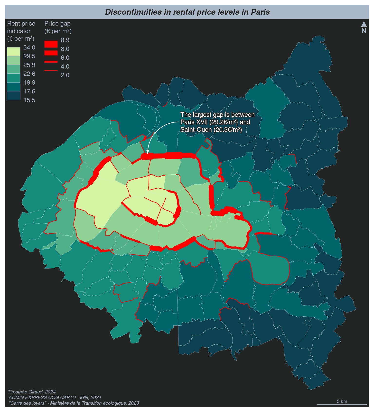
com_bo$diff <-abs(com_bo$loypredm2 - com_bo$loypredm2.1)# set a cartographic thememf_theme(x ="darkula",mar =c(.5, .5, 2, .5),inner =FALSE,pos ="center",tab =FALSE)# 
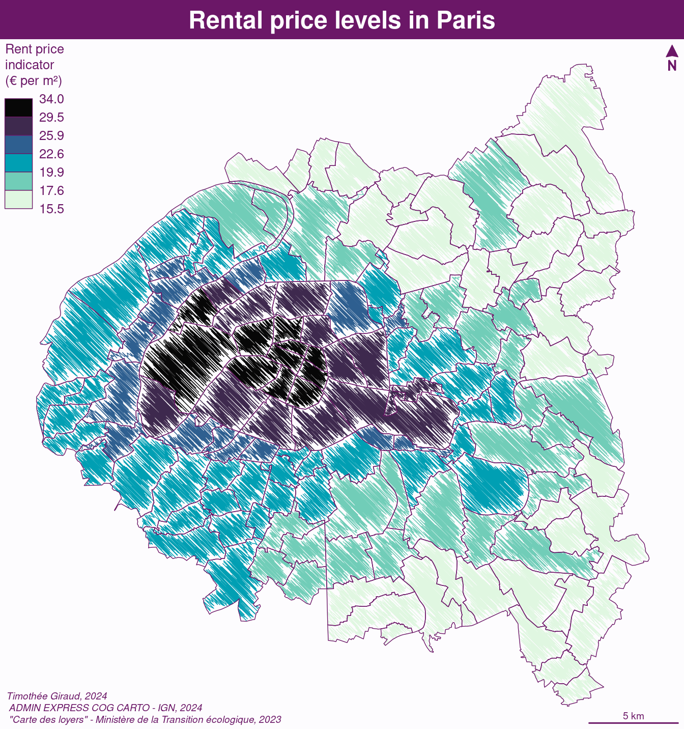
display a choropleth map of the rent price / m²mf_map(x = com, var ="loypredm2", type ="choro",breaks ="ckmeans", nbreaks =6, pal ="Emrld", rev = T,border ="grey90", lwd = .2,leg_title ="Rent price\nindicator\n(€ per m²)",leg_val_cex = .8, leg_val_rnd =1, leg_pos ="topleft")# display discontinuitiesmf_map(x = com_bo[com_bo$diff >=2, ], var ="diff", type ="grad",breaks =c(2, 4, 6, 8, 8.9), lwd =c(1, 4, 10, 14), col ="red",leg_title ="Price gap\n(€ per m²)",leg_val_rnd =1, leg_pos ="topleft", leg_adj =c(8, 0),leg_val_cex = .8)# Layout elementsmf_arrow("topright")mf_credits(txt =paste('Timothée Giraud, 2024\n','ADMIN EXPRESS COG CARTO - IGN, 2024\n','"Carte des loyers" - Ministère de la Transition écologique, 2023' ))mf_title("Discontinuities in rental price levels in Paris")mf_annotation(x = com_bo[order(com_bo$diff, decreasing =TRUE), ][1, ],txt =paste0("The largest gap is between\nParis XVII (29.2€/m²) and\n", "Saint-Ouen (20.3€/m²)"),halo =TRUE, s =2, col_arrow ="white", col_txt ="white",pos ="topright")mf_scale(5)
Colored pencil maps with mf_get_pencil()
mf_get_pencil() transforms POLYGONS or MULTIPOLYGONS geometries in MULTILINESTRINGS geometries. This function creates a layer that mimicks a pencil drawing pattern. The following code details how to use the function:
# transform the POLYGON layer in a MULTILINESTRING layercomx <-mf_get_pencil(com, size =250)# set a cartographic thememf_theme("candy")# display the map as a choropleth mapmf_map(x = comx, var ="loypredm2", type ="choro",breaks ="ckmeans", nbreaks =6, pal ="Mako",leg_title ="Rent price\nindicator\n(€ per m²)",leg_val_cex = .8, leg_val_rnd =1, leg_pos ="topleft")mf_map(com, add = T, col =NA, border =getOption("mapsf.fg"))# Layout elementsmf_arrow("topright")mf_credits(txt =paste('Timothée Giraud, 2024\n','ADMIN EXPRESS COG CARTO - IGN, 2024\n','"Carte des loyers" - Ministère de la Transition écologique, 2023' ))mf_title("Rental price levels in Paris")mf_scale(5)
Bug fixes and improvements
2 lines titles
A fix has made it easier to create titles on two lines.
# set a suitable cartographic thmemf_theme(bg ="grey90", fg ="black", mar =c(0,0,2.2,0), inner =FALSE, line =2.2, cex =1, pos ="left")mf_map(com)# display the titlemf_title("This title is easlily\ndisplayed on 2 lines")
A better north arrow
The north arrow has been redesigned. It is now possible to change its size (cex), fine-tune its position (adj) or use a true north azimuth (align).
mf_theme("jsk")# use a projection that will produce a map where the north is not at the topcom_usa <-st_transform(com, "EPSG:32119")mf_map(com_usa)mf_arrow(pos ="topleft", align = com_usa, cex =2)mf_graticule(com_usa, pos =c("bottom", "left"),add =TRUE)mf_title(txt ="A better north arrow")
New classification methods
The “Q6” and “ckmeans” methods have been added to the mf_get_breaks() function.
The “Q6” method has also been added, it’s a variation of the “q6” method.
The “jenks”, “fisher” and “ckmeans” methods are based on the same concept of natural breaks and produce similar groupings.
The “jenks” method produces class boundaries that fall on data points and is slow.
The “fisher” method produces class boundaries placed more conveniently between data points, and is faster than the “jenks” method.
The “ckmeans” method produces the exact same class boundaries as the “fisher” method, but is much faster. It uses the optimal univariate k-means method from the Ckmeans.1d.dp package (Wang and Song 2011). If the “ckmeans” method is selected but the Ckmeans.1d.dp package is not installed then the “fisher” method is used.
The relative speeds of these three methods may vary depending on the number of data points and the number of classes.
“fisher” vs. “ckmeans”
Jenks isn’t even included due to the prohibitive amount of time it would take.
Wang, Haizhou, and Mingzhou Song. 2011. “Ckmeans.1d.dp: Optimal k-Means Clustering in One Dimension by Dynamic Programming.”The R Journal 3 (2): 29–33. https://doi.org/10.32614/RJ-2011-015.